Robinson Crusoe Island in 3D: the real island, in real time, in the browser

The challenge

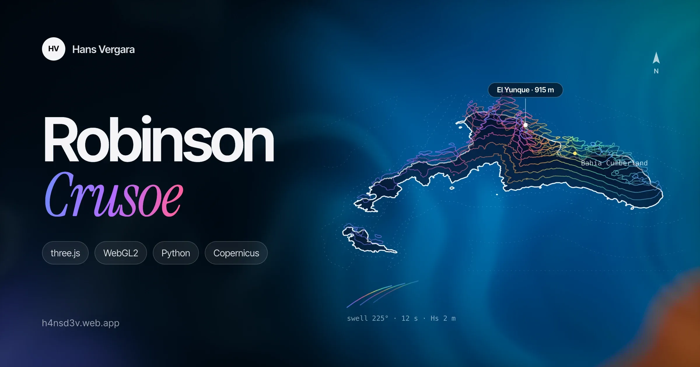
Robinson Crusoe Island lies about 670 km off mainland Chile, in the Juan Fernández archipelago: basalt cliffs dropping into the Pacific, ravines covered in native forest, and El Yunque, 915 m high, towering over Cumberland Bay. I set out to bring it to the browser as it really is: photorealistic, with true north and scale, explorable from a view of the whole archipelago down to the edge of a beach, at 60 frames per second on a MacBook Air.

One rule guided the whole project: no invented geography. Relief, coastline, bathymetry and the position of every place come from real data. Procedural content is only allowed as detail below the data’s resolution: the shape of a wave, the texture of a rock, the mesh of a tree.

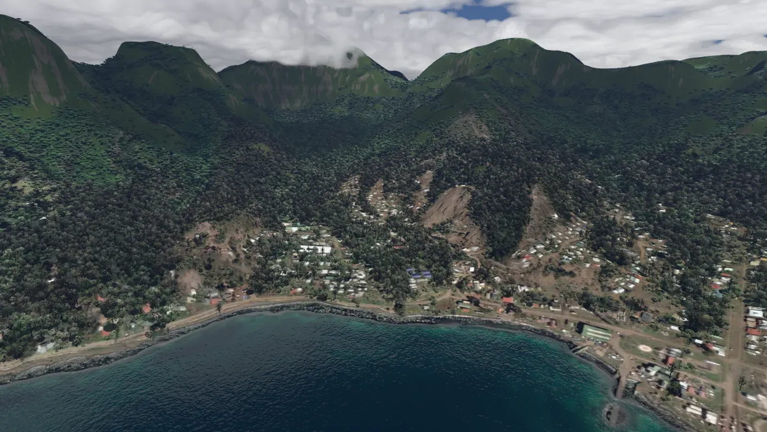
Cumberland Bay and the village of San Juan Bautista under El Yunque. The camera matches the exact position of a reference drone photo.

From satellites to the scene

Half the work happens before the first pixel is drawn, in a Python data pipeline. A shared contract (SPEC.md) fixes the coordinate system, a local scaled Web Mercator projection with under 0.1 % error, and the formats the pipeline and the renderer must follow to the letter.

• Relief: the Copernicus GLO-30 elevation model (30 m) is resampled to a ~4 m master grid with a B-spline approximation that never overshoots at cliffs. GMRT and GEBCO bathymetry is eased into the coastline with a Poisson fit.
• Imagery: a cloud-free Sentinel-2 composite defines the true surface colour (albedo). The best Esri captures, historical ones included, are fused on top of it: chosen for the least cloud, shadow and haze, colour-matched and feathered at the seams.
• Coastline: a classifier on the imagery refines the coast to about 2 m and yields the distance to the coast, beaches, forest, exposure to the south-west swell and the south-east wind, and the type of shore: sand, boulders or cliff.
• Fine relief: where there are morning and afternoon captures, shape-from-shading recovers the ravines the 30 m model misses, and islet heights are measured from the length of their shadows.
• The seabed: the island shelf is calibrated on a curious landmark, the wreck of the German cruiser SMS Dresden, scuttled in 1915 about 70 m deep off Cumberland.

Everything ends up in a tile pyramid, from the overview (z11) to 4 m detail (z17–z18). Heights are stored as 65×65 tiles with bit-identical borders, so no cracks appear between levels. Imagery is compressed as ASTC, which cuts GPU memory by four.

Rendering in the browser

The renderer is written in TypeScript on three.js and WebGL2, organised as independent features: sky, terrain, ocean, clouds and vegetation.

• Terrain: a level-of-detail quadtree with geomorphing, so nothing pops as you get closer. Tiles load by screen-space error priority, with extra detail right at the coastline, where errors show the most.
• Sky: a physically based atmosphere (Hillaire 2020) and a sun computed for the real date and time on the island.
• Ocean: the open sea is a GPU FFT (Tessendorf) with four cascades and a JONSWAP spectrum: the 12 s south-west swell plus the south-east wind sea. Near the coast, waves refract over the real bathymetry by solving the eikonal equation with fast sweeping: they turn toward the shore, shorten, wrap around headlands and break according to the depth. Foam appears where the satellite imagery shows breakers.
• Clouds: volumetric, with an orographic field computed from mountain-wave theory (Smith 2004) that builds cloud banks over the mountain ridge. Their shadows fall on the terrain and the sea.
• Vegetation: the land-cover map decides where the forest is. Full tree meshes are drawn near the camera and hemi-octahedral impostors in the mid range: over 80,000 in the Cumberland view. With cascaded shadows and wind.
• Final image: auto-exposure that works like a camera’s light meter, a photographic tone curve, white balance and dynamic resolution to hold the frame rate.

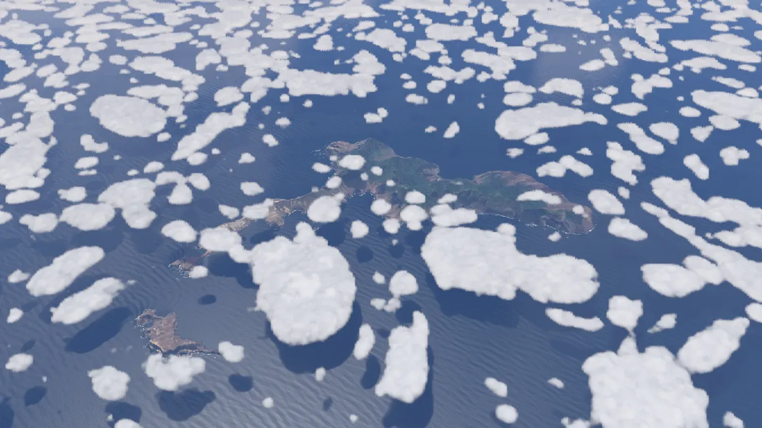
Overview of the archipelago: Robinson Crusoe, Santa Clara to the south-west and volumetric clouds casting their shadows on the ocean.

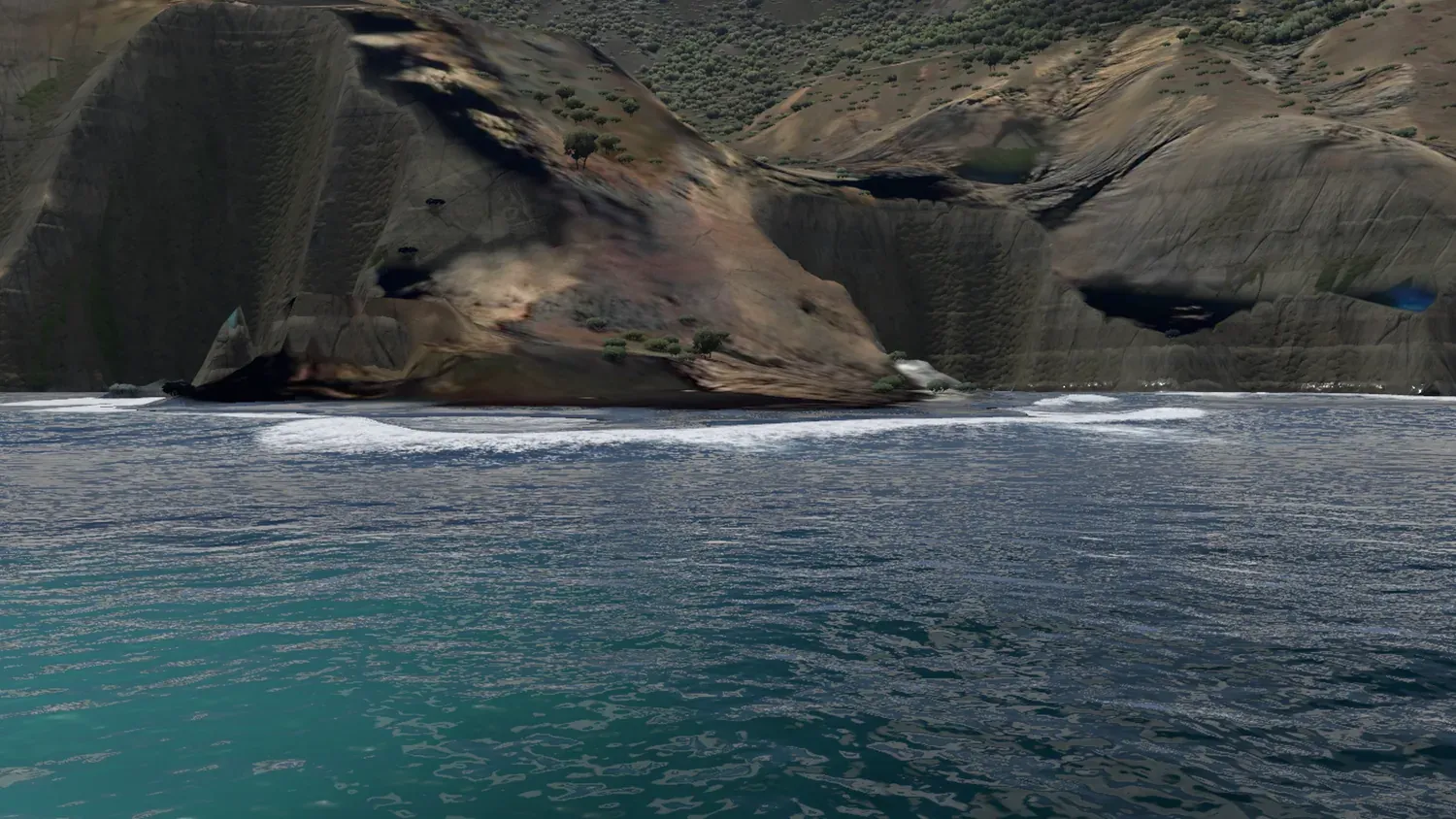
Breakers at Bahía Chupones: the waves refract over the real bathymetry and break according to the depth.

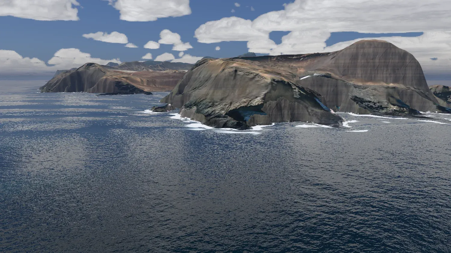
The cliffs of Punta Isla, in the south-west: the relief comes from the real elevation model, refined where the imagery allows it.

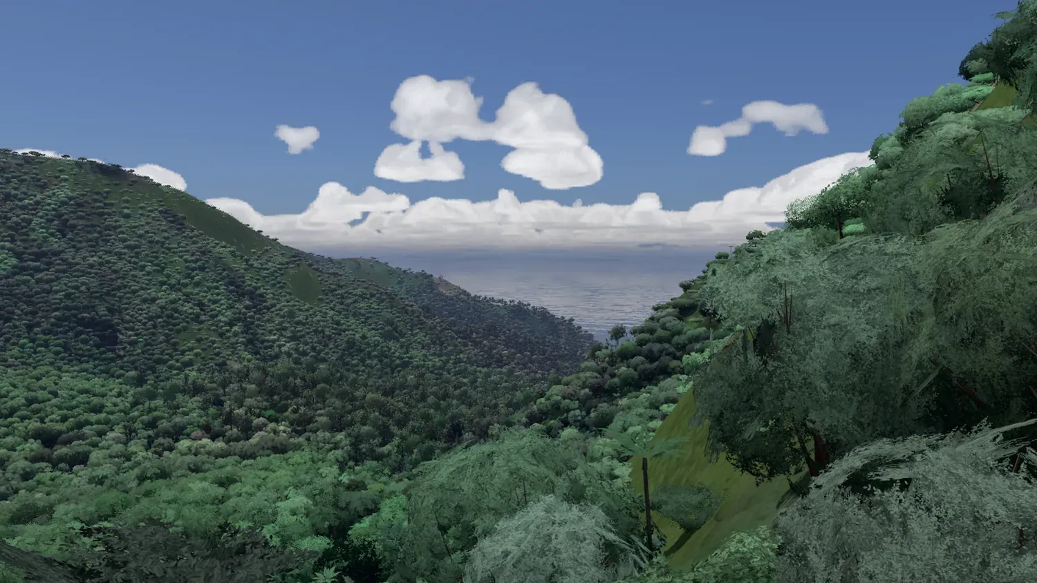
Native forest below El Yunque: full tree meshes near the camera and impostors in the mid range, placed from the land-cover map.

Performance

The target was 60 fps on a MacBook Air M3, which has no fan and heats up under sustained load. I learned to measure before optimising: on ANGLE/Metal, GPU timer queries return overlapping intervals and are useless. So the test harness measures the cost of each part by elimination, switching them off one by one within the same page. In Cumberland Bay, at 1600×900, a full frame takes about 15 ms. Dynamic resolution and ASTC textures cover the rest.

What I learned

• An explicit data contract is gold. With the specification as the single source of truth, the pipeline and the renderer could evolve separately without breaking each other.
• Physics buys realism for free. Wave refraction, the atmosphere or clouds over the relief computed with their real physics look right in situations I never tested by hand.
• AI-assisted development. I built the project with Claude Code as a copilot. What mattered most was writing precise specifications and checking every result with screenshots and measurements, rather than trusting the first answer.

The project currently runs locally: part of the satellite imagery it uses (Esri World Imagery) is licensed for personal use, so a public release would need to replace it.

Stack

• Renderer: TypeScript, three.js, WebGL2, Web Workers, Vite
• Data pipeline: Python, NumPy, SciPy, scikit-image, rasterio
• Data: Copernicus DEM GLO-30, Sentinel-2 L2A, Esri World Imagery, GMRT, GEBCO, OpenStreetMap
• Tools: Playwright (screenshot and performance harness), Claude Code

---

Images rendered in real time by the project. Satellite imagery: Esri World Imagery (Esri, Maxar, Earthstar Geographics and the GIS User Community); contains modified Copernicus Sentinel-2 data; Copernicus DEM GLO-30 © DLR e.V. 2010–2014 and © Airbus Defence and Space GmbH 2014–2018; GMRT and GEBCO bathymetry; © OpenStreetMap contributors.